Quick start
The histpy library provides a Histogram class which is, essentially, an array with axes attached defining the bin boundaries. The histpy library class is loosely based on ROOT’s histogram but using a more pythonic interface.
The histpy library supports:
Histograms with an arbitrary number of dimensions.
Numpy-like element indexing.
Multiple operations: projection, slicing, addition, multiplication, concatenation, rebinning, fitting, interpolation and plotting.
Tracking of under and overflow contents along each axes.
Weighted histograms.
Automatic error propagation.
Astropy’s units, both for the histogram contents and the axis edges.
Spherical coordinates axes, using the HEALPix grid.
Sparse contents
I/O to/from HDF5 files.
Native support for astropy
TimeandTimeDeltaobjects.
This is an overview of all of these features. More details can be found in the API documentation.
Initialization
A Histogram object is defined by a series of bin edges (one more than the number of bins)
[1]:
from histpy import Histogram
import numpy as np

h = Histogram(np.linspace(-5,5,101))
The edges become part of the histograms’ Axis
[2]:
print("Number of bins:".format(h.axis.nbins))
print("Bin centroids: {}".format(h.axis.centers))
Number of bins:
Bin centroids: [-4.95 -4.85 -4.75 -4.65 -4.55 -4.45 -4.35 -4.25 -4.15 -4.05 -3.95 -3.85
 -3.75 -3.65 -3.55 -3.45 -3.35 -3.25 -3.15 -3.05 -2.95 -2.85 -2.75 -2.65
 -2.55 -2.45 -2.35 -2.25 -2.15 -2.05 -1.95 -1.85 -1.75 -1.65 -1.55 -1.45
 -1.35 -1.25 -1.15 -1.05 -0.95 -0.85 -0.75 -0.65 -0.55 -0.45 -0.35 -0.25
 -0.15 -0.05  0.05  0.15  0.25  0.35  0.45  0.55  0.65  0.75  0.85  0.95
  1.05  1.15  1.25  1.35  1.45  1.55  1.65  1.75  1.85  1.95  2.05  2.15
  2.25  2.35  2.45  2.55  2.65  2.75  2.85  2.95  3.05  3.15  3.25  3.35
  3.45  3.55  3.65  3.75  3.85  3.95  4.05  4.15  4.25  4.35  4.45  4.55
  4.65  4.75  4.85  4.95]
Specify the edges for multiple axes to get a histogram with an arbitrary number of dimensions. You can label the axes.
[3]:
h2D = Histogram([np.linspace(10,30,201), np.linspace(0,5,101)], labels = ['x','y'])

for axis in h2D.axes:
    print("Axis '{}' has {} bins".format(axis.label, axis.nbins))
Axis 'x' has 200 bins
Axis 'y' has 100 bins
Filling
You can fill the histogram entry by entry
[4]:
np.random.seed(0)
for x in np.random.normal(size = 10000):
    h.fill(x)
Or all at once:
[5]:
x = np.random.normal(loc = 21, scale = 2, size = 10000)
y = np.random.normal(loc = 3, scale = .2, size = 10000)

h2D.fill(x,y)
The latter is recommended for performance reasons.
Plotting
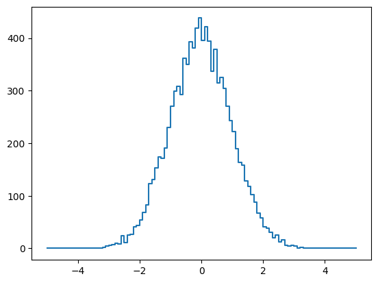
You can plot 1D and 2D histograms using plot().
[6]:
h.plot();
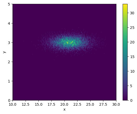
2D histograms can also be plotted:
[7]:
h2D.plot();
Plotting histograms with a number of dimensions >=3 is not currently supported.
The histograms are plotted using matplotlib. In the case of 1D histograms, plot() is a wrapper for `errorbar() <https://matplotlib.org/stable/api/_as_gen/matplotlib.pyplot.errorbar.html>`__. For 2D histogram, it uses `pcolormesh() <https://matplotlib.org/stable/api/_as_gen/matplotlib.pyplot.pcolormesh.html>`__.
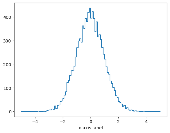
By default, plot() creates a new set of matplotlib axes. These are returned together with the plot handle so you can use to further customize the plot:
[8]:
ax,plot = h.plot()

ax.set_xlabel("x-axis label");
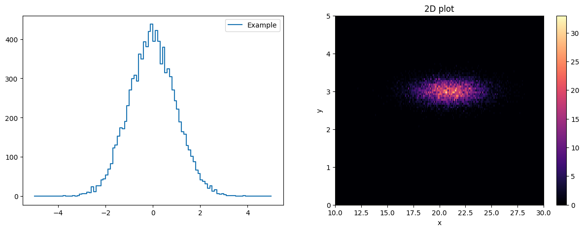
Or, alternatively, you can pass the matplotlib axes where you want the plot. e.g.
[9]:
import matplotlib.pyplot as plt

fig,ax = plt.subplots(ncols = 2, figsize = [15,5])

h.plot(ax[0], label = "Example")
ax[0].legend()

h2D.plot(ax[1], cmap = 'magma')
ax[1].set_title("2D plot");
The method draw() is an alias for plot() kept for backwards compatibility.
Underflow and overflow tracking
The number of samples beyond an axis range can be tracked by setting track_overflow = True. Despite the abbreviated name, it tracks underflow values as well.
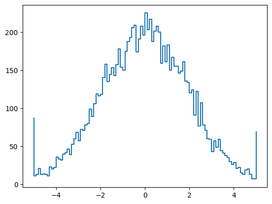
When plotting 1D histogram, the underflow and overflow are represented by “spikes” on either end:
[10]:
h = Histogram(np.linspace(-5,5,101), track_overflow = True)

h.fill(np.random.normal(scale = 2, size = 10000)) # Broader than the previous example

h.plot()
[10]:
(<Axes: >, <ErrorbarContainer object of 3 artists>)
While underflow and overflow contents are only plotted for 1D histograms, they are tracked for any number of dimensions. The underflow and overflow bins “surround” the histogram’s contents, adding two additional entries to each dimension:
[11]:
h2D = Histogram([np.linspace(10,30,4), np.linspace(0,5,5)],
                track_overflow = True)

h2D[:] = 1 # The indexing will be explained in the following section

print(h2D.full_contents)
[[0. 0. 0. 0. 0. 0.]
 [0. 1. 1. 1. 1. 0.]
 [0. 1. 1. 1. 1. 0.]
 [0. 1. 1. 1. 1. 0.]
 [0. 0. 0. 0. 0. 0.]]
Indexing
For the most part, the contents of a histogram can be accessed the same way as a numpy array
[12]:
# Accessing the contents on a bin
h[50]
[12]:
np.float64(225.0)
[13]:
# A range
h[50:60]
[13]:
array([225., 203., 217., 188., 201., 208., 200., 159., 182., 161.])
[14]:
# A list of bins
h[[0,50,80]]
[14]:
array([ 11., 225., 43.])
[15]:
# Boolean mask
h[h > .9*np.max(h)]
[15]:
array([206., 209., 208., 225., 203., 217., 208.])
However, the -1 bin DOES NOT correspond to the last bin, but rather to the underflow bin. Similarly, the bin number equal to the total number of bins is the overflow bin.
[16]:
# Underflow
h[-1]
[16]:
np.float64(87.0)
[17]:
# Overflow
h[h.nbins]
[17]:
np.float64(69.0)
The special constant end can be used to access any bin relative to the last one, e.g.
h[h.end-10] <-> h[h.nbins-10]
This is specially useful for multi-dimensional histograms, where the property nbins is not a number, but a sequence. Use end instead and it will be automatically replaced by the number of bins in that dimension
[18]:
# Here we initialize a histogram with non-zero contents
# All bin contents equal 1, except the under/overflow bins
# You can initialize them as well, but in this case they are empty
h = Histogram([np.linspace(0,6,7), np.linspace(0,4,5)],
              contents = np.ones((6,4)),
              labels = {'x', 'y'},
              track_overflow = True)

print("Number of dimensions: {}".format(h.ndim))
print("Number of bins on each axis: {}".format(h.nbins))

# DO NOT do this.
# h[:, h.nbins-1] is equivalent to h[:, [5,3]] and will raise an out-of-bounds exception (in this case)
# h[:, h.nbins-1]

# DO this
print("Last y-bin: {}".format(h[:, h.end-1]))
Number of dimensions: 2
Number of bins on each axis: [6 4]
Last y-bin: [1. 1. 1. 1. 1. 1.]
The implicit index for unspecified dimensions is :, which doesn’t include underflow/overflow:
[19]:
h[0] # = h[0,:]
[19]:
array([1., 1., 1., 1.])
If you want to include these special bins for all the reminding axes use ... (the Ellipsis object)
[20]:
h[0,...] # = h[0, -1:h.end+1]
[20]:
array([0., 1., 1., 1., 1., 0.])
The following aliases are provided just for convenience and readability
h.uf = -1
h.of = h.end
h.all = slice(-1,h.end+1) # i.e. h[h.all] -> h[-1:h.end+1]
NOTE: Negative indices DO NOT correpond to bins counting from the end. h[-1] corresponds to the underflow bin and other negative values will raise an IndexError. Use instead e.g. h[h.nbins-1] or h[h.end-3].
Attempting to access an underflow/overflow bin when they are not tracked (see track_overflow()) will result in an IndexError. If the under/overflow is not tracked, then
h.all = slice(0,h.end) # i.e. h[h.all] -> h[0:h.end]
Weighted histograms
You can also fill the histograms using weighted data. If you care about statistical errors though you’ll want to set sumw2=True while initializaing the histogram. The histogram will then save the sum of the weights squared for each bin (\(\sum w_i^2\)). The bin errors will then be \(\sqrt{\sum w_i^2}\) (assuming Gaussian statistics) as opposed to \(\sqrt{N}\).
[21]:
h = Histogram(np.linspace(-2,2, 100), sumw2 = True)

nsamples = 10000
x = np.random.uniform(low=-3, high=3, size=nsamples)

# You can use warn_overflow = False to supress the warning below
h.fill(x, weight = np.exp(-x*x)/nsamples)

h.plot();
fill() discarded one or more values due to out-of-bounds coordinate in a dimension without under/overflow tracking
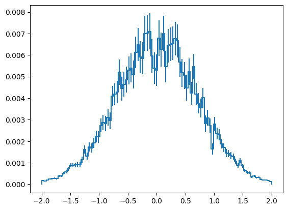
The individual stored values can be accessed using sumw2[]
[22]:
print("Bin {}: {:.2e} +/- {:.2e}".format(50, h[50], np.sqrt(h.sumw2[50])))
Bin 50: 6.79e-03 +/- 8.23e-04
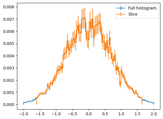
Slice and project
You might have noticed that when you slice a histogram using [] the output is an array with the corresponding contents. By using slice[] you can instead obtain a Histogram object, which contains both contents and axes
[23]:
ax,plot = h.plot(label = "Full histogram")

h.slice[10:90].plot(ax, label = "Slice")

ax.legend();
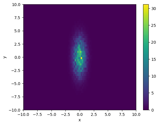
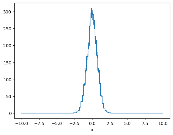
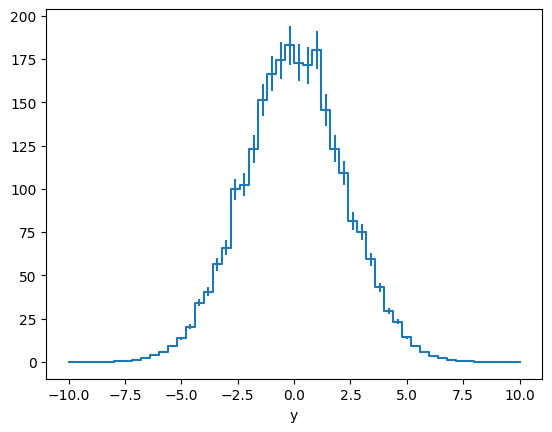
You can also project a multi-dimensional histogram onto one or more axes, reducing the number of dimensions
[24]:
x_edges = np.linspace(-10,10,101)
y_edges = np.linspace(-10,10,51)

h = Histogram([x_edges, y_edges], labels = ['x','y'], sumw2 = True)

x = np.random.uniform(low=-10, high=10, size=100000)
y = np.random.uniform(low=-10, high=10, size=100000)

h.fill([x,y], weight = np.exp(-x*x-y*y/10))

h.plot()

h.project('x').plot()

h.project('y').plot();
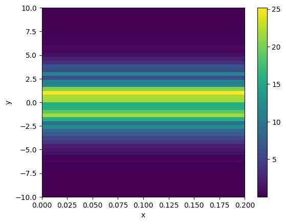
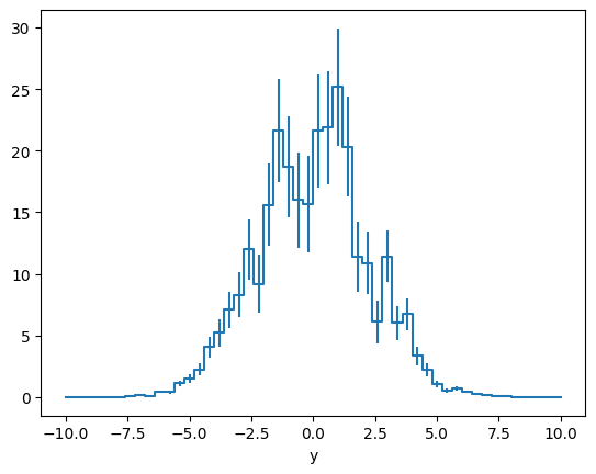
Because slice always returns a histogram of the same dimensionality as the original, no matter the number of selected bins, if you want to get a “cross section” then you need to slice and project
[25]:
h.slice[50].plot()

h.slice[50].project('y').plot();
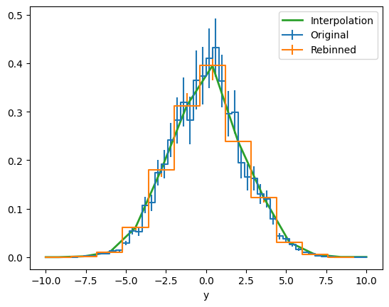
Interpolation and rebinning
Basic rebinning and linear interpolation is also provided
[26]:
# 1D example

# First we take a slice as before
h_slice = h.slice[30:40].project('y')

ax,plot = h_slice.draw(label = "Original")

# Rebining sums N bins together.
# Here we divide by N to obtain the average
h_rebin = h_slice.rebin(4)/4

h_rebin.draw(ax, label = "Rebinned")

# Interpolating at the original bin centroids
x = np.linspace(-10,10,51)

ax.plot(x, h_rebin.interp(x), linewidth = 2, label = "Interpolation");

ax.legend()
[26]:
<matplotlib.legend.Legend at 0x1320d01d0>
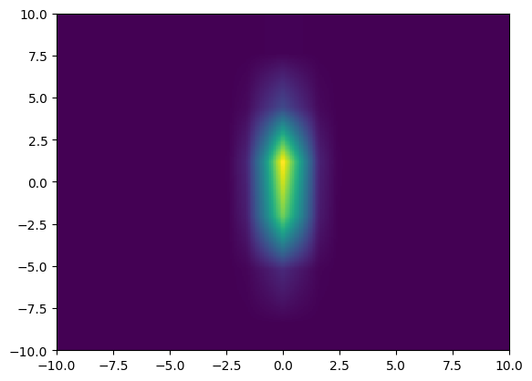
[27]:
# 2D example

# Rebinning
h_rebin = h.rebin(4,8)

# e.g Interpolating a 2D histogram
x = np.linspace(-10,10,301)
y = np.linspace(-10,10,301)
X,Y = np.meshgrid((x[1:]+x[:-1])/2, (y[1:]+y[:-1])/2)

plt.pcolormesh(x,y, h_rebin.interp(X,Y));
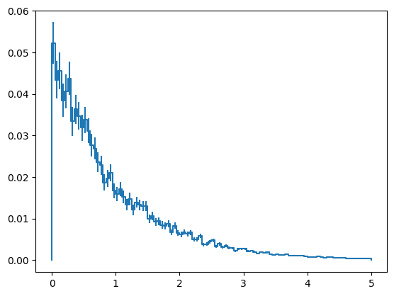
Arithmetic operations
Histogram supports arithmethic operations (+, -, *, /) with other Histogram objects, scalars, and arrays of an appropiate size. Make sure to set sumw2=True during initialization so the errors are propagated appropiately.
[28]:
# e.g. normalizing a histogram
h = Histogram(np.linspace(0,5, 101), sumw2 = True)

x = np.random.uniform(0,5, size = 10000)
h.fill(x, weight = np.exp(-x))

h /= np.sum(h)

h.draw();
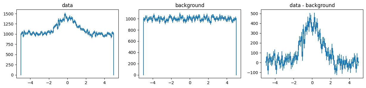
[29]:
# e.g. substracting a background

fig,ax =  plt.subplots(ncols = 3, figsize = [15,3])

# Source + background histogram
h = Histogram(np.linspace(-5,5, 101), sumw2 = True)

x = np.random.normal(size = 10000)
h.fill(x)

bkg = np.random.uniform(-5,5, size = 100000)
h.fill(bkg)

h.draw(ax[0])

ax[0].set_title("data")

# Background only histogram
h_b = Histogram(np.linspace(-5,5, 101), sumw2 = True)

bkg = np.random.uniform(-5,5, size = 100000)
h_b.fill(bkg)

h_b.draw(ax[1])

ax[1].set_title("background")

# Brackground-subtrated histogram

h_s = h-h_b
h_s.draw(ax[2])

ax[2].set_title("data - background");
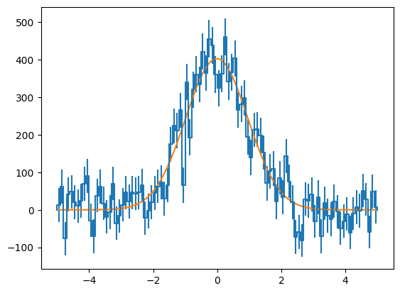
Fitting
A convenient wrapper of scipy’s curve_fit is provided. All user parameters are passed along together with the histogram’s data.
[30]:
# Define a function to fit
def f(x, N, x0, var):
    return N*np.exp(-(x-x0)**2/2/var)

# Histogram will pass the initial guess (p0) to scipy curve_fit
sol,cov = h_s.fit(f, p0 = [500,1,2])

# Plot result
x = np.linspace(-5,5,100)

ax,_ = h_s.draw()

ax.plot(x, f(x, *sol));
Disk I/O
Lastly, you can save the histogram to disk as an HDF5 file
[31]:
h.write("hist.h5", overwrite=True)
[32]:
h2 = Histogram.open("hist.h5")
[33]:
h == h2
[33]:
True
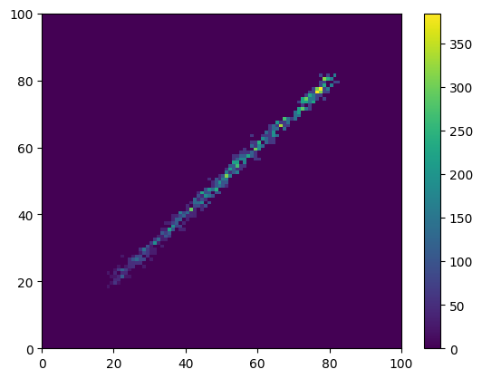
Sparse histograms
Sparse histogram are useful when most of the bins will be empty. This allows to handle a large number of bins or dimensions that would otherwise might be resource prohibitive.
For example, let’s create an spase histogram with 10^12 bins:
[34]:
h = Histogram([np.linspace(0,100,101) for n in range(6)], sparse = True)
Sparse histogram are handled the same way as regular dense histogram, and for the most part you don’t have to write code specific for them.
In this example we’ll fill the histogram with 6 fully corelated variables, each with a small statistical error:
[35]:
nsamples = 1000

h.fill(np.random.uniform(0,100,nsamples) + np.random.normal(size = (h.ndim,nsamples)),
      warn_overflow = False)
You can then perform any operation as usual:
[36]:
# Slice along the 5th axis
h = h.slice[{4:slice(20,80)}]

# Linear weight along the 3rd axis
h *= h.expand_dims(h.axes[2].centers, 2)

# Project onto the first 2 axes
h = h.project(0,1)

h.plot()
[36]:
(<Axes: >, <matplotlib.collections.QuadMesh at 0x136dd1350>)
The main difference is that sparse histograms return SparseArrays instead of regular numpy arrays
[37]:
type(h.contents)
[37]:
sparse._coo.core.COO
You can transform a sparse histogram into a regular one using to_dense()
[38]:
type(h.to_dense().contents)
[38]:
numpy.ndarray
NOTE: When working with sparse histograms, and for optimal efficiency, complete the filling process before performing operations —e.g. projections, slices, arithmetics, etc. There is an overhead required to prepare the histogram for contents modification.
NOTE: SparseArray do not yet fully supports numpy’s advance indexing —i.e. using an index array. Accessing the contents with a one-dimensional array works —e.g. h[[0,3,7]], but multiple dimensional array —e.g. h[[[0,3,7]]]— and setting multiple bins —e.g. h[[0,3,7]] = 1— does not.
Units
Both Histogram and Axis support astropy’s units for the contents and edges, respectively:
[39]:
import astropy.units as u

h = Histogram(np.linspace(0,100,100) * u.cm)

# The unit's conversion is handled internally
h.fill(np.random.uniform(0, 1, 10000) * u.m)

# The histogram contents can also have units,
# which are updated when arithmethic operations are applied
h /= h.axis.widths

print(f"Axis units = {h.axis.unit}")
print(f"Histogram contents units = {h.unit}")
Axis units = cm
Histogram contents units = 1 / cm
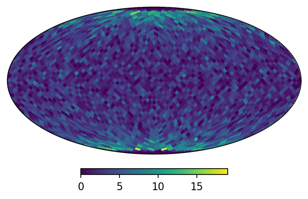
HealpixAxis
The HealpixAxis is class inherits from the general Axis and mhealpy’s HealpixBase. It allows to bin data representing directions in spherical coordinates. In this case, the bins correspond to pixels in a HEALPix grid.
Histograms using HealpixAxis are plotted using WCSAxes. See also mhealpy’s plotting documentation.
[40]:
from histpy import HealpixAxis
from astropy.coordinates import UnitSphericalRepresentation

# nside must be a power of 2.
# The pixel size is approximately 60deg/nside
h_map = Histogram(HealpixAxis(nside = 16))

# Fill with uniform distributions in longitude and latitude,
# which is NOT an uniform distribution in the sphere
nsamples = 10000
lon = np.random.uniform(  0,360,nsamples)*u.deg
lat = np.random.uniform(-80, 80,nsamples)*u.deg
points = UnitSphericalRepresentation(lon = lon, lat = lat)

h_map.fill(points)

# Mollweide projection (by default)
h_map.plot();
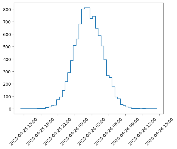
TimeAxis and TimeDeltaAxis
The TimeAxis and TimeDeltaAxis inherit from the general Axis and can handle natively astropy’s Time and TimeDelta object.
The main differences compared to using a regular Axis with time unit are:
TimeAxisandTimeDeltaAxishandle the transformation between different time formats and systems.TimeandTimeDeltainternally store two 64-bit values to achieve sub-ns precision at any point in the history of the Universe.TimeAxisis plotted using matplotlib’s date formatter for more meaningful tick labels.
If you provide a Time object as edges, Histogram will automatically use TimeAxis.
[2]:
from astropy.time import Time

t0 = Time.now()
edges = t0 + np.linspace(0*u.day,1*u.day) # This is also a Time object

h = Histogram(edges) # Automatically uses TimeAxis

random_times = t0 + np.random.normal(loc = .5, scale = .1, size = 10000)*u.day
h.fill(random_times)

ax,plot = h.plot()

# Optional: Format axes
import matplotlib.dates as mdates
ax.tick_params(axis='x', labelrotation=45)
ax.xaxis.set_major_formatter(mdates.DateFormatter('%Y-%m-%d %H:%M'))
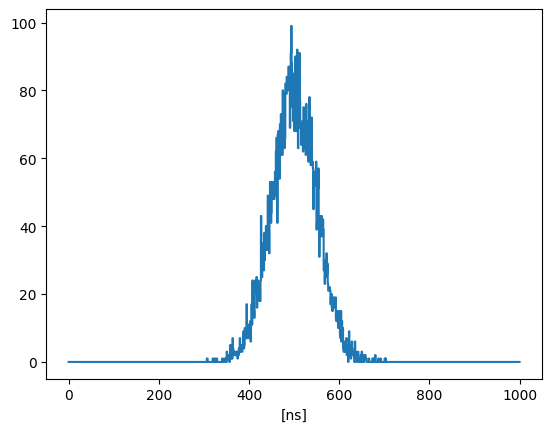
You can convert TimeAxis to a TimeDeltaAxis by subtracting a reference time, and viceversa:
[3]:
t0 = Time.now()

# Keeps sub-ns bins
edges = t0 +  np.linspace(0*u.us,1*u.us,1000)

h = Histogram(edges)

random_times = t0 + np.random.normal(loc = 500, scale = 50, size = 10000)*u.ns
h.fill(random_times)

# Get a TimeDeltaAxis by subtracting a time
h.axis = h.axis - t0

# Optional: transform to a regular Axis with units
h.axis = h.axis.to(u.ns)

ax,plot = h.plot()
[ ]:
[ ]: